In this document we discuss the spatially-adaptive finite-element-based solution of the 3D Helmholtz equation in cylindrical polar coordinates, using a Fourier-decomposition of the solution in the azimuthal direction.
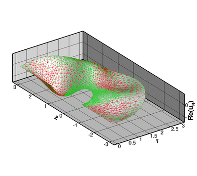
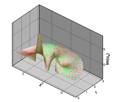
This solution corresponds to the superposition of several outgoing waves that emerge from the unit sphere.
The two plots below show a comparison between the exact and computed solutions for  , a Fourier wavenumber of
  , and a (squared) Helmholtz wavenumber of
  .
.
shows the main differences required to discretise the computational domain with an adaptive, unstructured mesh:
#include <complex>
#include <cmath>
#include "generic.h"
#include "fourier_decomposed_helmholtz.h"
#include "meshes/triangle_mesh.h"
#include "oomph_crbond_bessel.h"
using namespace oomph;
using namespace std;
{
std::complex<double>
I(0.0,1.0);
{
{
}
}
{
{
for (
unsigned i=0;
i<
nr;
i++)
{
for (
unsigned j=0;
j<
nz;
j++)
{
<<
uu.real() <<
" " <<
uu.imag() <<
"\n";
}
}
}
}
}
{
std::complex<double>
I(0.0,1.0);
{
{
}
}
{
flux=std::complex<double>(0.0,0.0);
{
}
}
}
template<class ELEMENT>
{
public:
{
{
}
}
private:
{
{
}
}
#ifdef ADAPTIVE
#else
#endif
};
template<class ELEMENT>
{
{
delete_face_elements(Helmholtz_outer_boundary_mesh_pt);
}
delete_face_elements(Helmholtz_inner_boundary_mesh_pt);
}
template<class ELEMENT>
{
unsigned n_element = Bulk_mesh_pt->nelement();
{
}
create_flux_elements_on_inner_boundary();
{
create_outer_bc_elements();
}
}
template<class ELEMENT>
{
Trace_file.open("RESLT/trace.dat");
{
}
else
{
}
#ifdef ADAPTIVE
Bulk_mesh_pt->min_permitted_error()=0.00004;
Bulk_mesh_pt->max_permitted_error()=0.0001;
#else
#endif
Bulk_mesh_pt->output("mesh.dat");
Bulk_mesh_pt->output_boundaries("boundaries.dat");
{
Helmholtz_outer_boundary_mesh_pt=
create_outer_bc_elements();
}
Helmholtz_inner_boundary_mesh_pt=
new Mesh;
create_flux_elements_on_inner_boundary();
{
}
unsigned n_element = Bulk_mesh_pt->nelement();
{
}
}
template<class ELEMENT>
{
Helmholtz_outer_boundary_mesh_pt->setup_gamma();
unsigned nel=Helmholtz_outer_boundary_mesh_pt->nelement();
{
(Helmholtz_outer_boundary_mesh_pt->element_pt(
e));
Helmholtz_outer_boundary_mesh_pt->gamma_at_gauss_point(
el_pt));
{
for(
unsigned i=0;
i<
n;
i++)
{
}
<< std::endl;
}
}
}
template<class ELEMENT>
{
cout <<
"Norm of solution: " <<
sqrt(
norm) << std::endl << std::endl;
Bulk_mesh_pt->compute_norm(
norm);
Trace_file <<
norm << std::endl;
{
}
}
template<class ELEMENT>
{
unsigned n_element = Bulk_mesh_pt->nboundary_element(
b);
{
Bulk_mesh_pt->boundary_element_pt(
b,
e));
}
}
template<class ELEMENT>
{
unsigned n_element = Bulk_mesh_pt->nboundary_element(
b);
{
Bulk_mesh_pt->boundary_element_pt(
b,
e));
}
}
{
{
{
for (
unsigned j=0;
j<=
n;
j++)
{
}
for (
unsigned j=0;
j<=
n;
j++)
{
}
for (
unsigned j=0;
j<=
n;
j++)
{
}
for (
unsigned j=0;
j<=
n;
j++)
{
}
}
}
{
{
for (
unsigned j=0;
j<=
n;
j++)
{
}
}
}
#ifdef ADAPTIVE
#else
#endif
{
#ifdef ADAPTIVE
#else
#endif
}
}
AnnularQuadMesh(const unsigned &n_r, const unsigned &n_phi, const double &r_min, const double &r_max, const double &phi_min, const double &phi_max)
~FourierDecomposedHelmholtzProblem()
Destructor (empty)
void actions_after_adapt()
Actions after adapt: Rebuild the mesh of prescribed flux elements.
void create_outer_bc_elements()
Create BC elements on outer boundary.
Mesh * Helmholtz_inner_boundary_mesh_pt
Mesh of face elements that apply the prescribed flux on the inner boundary.
void actions_after_newton_solve()
Update the problem after solve (empty)
void create_flux_elements_on_inner_boundary()
Create flux elements on inner boundary.
void actions_before_newton_solve()
Update the problem specs before solve (empty)
void doc_solution(DocInfo &doc_info)
Doc the solution. DocInfo object stores flags/labels for where the output gets written to.
void delete_face_elements(Mesh *const &boundary_mesh_pt)
Delete boundary face elements and wipe the surface mesh.
FourierDecomposedHelmholtzProblem()
Constructor.
FourierDecomposedHelmholtzDtNMesh< ELEMENT > * Helmholtz_outer_boundary_mesh_pt
Pointer to mesh containing the DtN boundary condition elements.
ofstream Trace_file
Trace file.
void check_gamma(DocInfo &doc_info)
Check gamma computation.
void actions_before_adapt()
Actions before adapt: Wipe the mesh of prescribed flux elements.
AnnularQuadMesh< ELEMENT > * Bulk_mesh_pt
Pointer to bulk mesh.
void actions_before_newton_convergence_check()
Recompute gamma integral before checking Newton residuals.
Namespace to test representation of planar wave in spherical polars.
void get_exact_u(const Vector< double > &x, Vector< double > &u)
Exact solution as a Vector of size 2, containing real and imag parts.
std::complex< double > I(0.0, 1.0)
Imaginary unit.
unsigned N_terms
Number of terms in series.
Namespace for the Fourier decomposed Helmholtz problem parameters.
unsigned N_terms
Number of terms in the exact solution.
unsigned Nterms_for_DtN
Number of terms in computation of DtN boundary condition.
double K_squared
Square of the wavenumber.
void exact_minus_dudr(const Vector< double > &x, std::complex< double > &flux)
Get -du/dr (spherical r) for exact solution. Equal to prescribed flux on inner boundary.
int N_fourier
Fourier wave number.
Vector< double > Coeff(N_terms, 1.0)
Coefficients in the exact solution.
std::complex< double > I(0.0, 1.0)
Imaginary unit.
void get_exact_u(const Vector< double > &x, Vector< double > &u)
Exact solution as a Vector of size 2, containing real and imag parts.
int main(int argc, char **argv)
Driver code for Fourier decomposed Helmholtz problem.
![\[
\nabla^2 {u_{N}}(r,z) + \left(k^2-\frac{N^2}{r^2}\right) u_N(r,z) = 0,
\ \ \ \ \ \ \ \ \ \ \ \ (1)
\]](form_0.png)
 is the azimuthal wavenumber, in the finite domain
 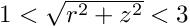 . We impose the Sommerfeld radiation condition at the outer boundary of the computational domain at
  , using a Dirichlet-to-Neumann mapping, and apply flux boundary condition on the surface of the unit-sphere (where
  ) such that the exact solution is given by
 ![\[
u_N(r,z)=u_N^{[exact]}(r,z)=\sum_{l=N}^{N_{\rm terms}}
h_{l}^{(1)}(k\sqrt{r^2+z^2}) \ P_{l}^{N}\left(\frac{z}{\sqrt{r^2+z^2}}\right).
\]](form_5.png)